04.03 概率统计方法
概率统计方法
简介
Python 中常用的统计工具有 Numpy, Pandas, PyMC, StatsModels 等。
Scipy 中的子库 scipy.stats 中包含很多统计上的方法。
导入 numpy 和 matplotlib:
1%pylab inline
Populating the interactive namespace from numpy and matplotlib
1heights = array([1.46, 1.79, 2.01, 1.75, 1.56, 1.69, 1.88, 1.76, 1.88, 1.78])
Numpy 自带简单的统计方法:
1print 'mean, ', heights.mean()
2print 'min, ', heights.min()
3print 'max, ', heights.max()
4print 'standard deviation, ', heights.std()
mean,  1.756
min,  1.46
max,  2.01
standard deviation,  0.150811140172
导入 Scipy 的统计模块:
1import scipy.stats.stats as st
其他统计量:
1print 'median, ', st.nanmedian(heights)    # 忽略nan值之后的中位数
2print 'mode, ', st.mode(heights)           # 众数及其出现次数
3print 'skewness, ', st.skew(heights)       # 偏度
4print 'kurtosis, ', st.kurtosis(heights)   # 峰度
5print 'and so many more...'
median,  1.77
mode,  (array([ 1.88]), array([ 2.]))
skewness,  -0.393524456473
kurtosis,  -0.330672097724
and so many more...
概率分布
常见的连续概率分布有:
- 均匀分布
- 正态分布
- 学生
t分布 F分布Gamma分布- ...
- 伯努利分布
- 几何分布
- ...
这些都可以在 scipy.stats 中找到。
连续分布
正态分布
以正态分布为例,先导入正态分布:
1from scipy.stats import norm
它包含四类常用的函数:
从正态分布产生500个随机点:
1x_norm = norm.rvs(size=500)
2type(x_norm)
numpy.ndarray
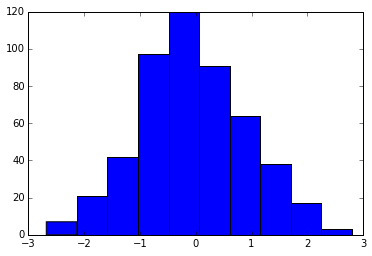
直方图:
1h = hist(x_norm)
2print 'counts, ', h[0]
3print 'bin centers', h[1]
counts,  [   7.   21.   42.   97.  120.   91.   64.   38.   17.    3.]
bin centers [-2.68067801 -2.13266147 -1.58464494 -1.0366284  -0.48861186  0.05940467
  0.60742121  1.15543774  1.70345428  2.25147082  2.79948735]
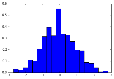
归一化直方图(用出现频率代替次数),将划分区间变为 20(默认 10):
1h = hist(x_norm, normed=True, bins=20)
在这组数据下,正态分布参数的最大似然估计值为:
1x_mean, x_std = norm.fit(x_norm)
2
3print 'mean, ', x_mean
4print 'x_std, ', x_std
mean,  -0.0426135499965
x_std,  0.950754110144
将真实的概率密度函数与直方图进行比较:
1h = hist(x_norm, normed=True, bins=20)
2
3x = linspace(-3,3,50)
4p = plot(x, norm.pdf(x), 'r-')

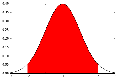
导入积分函数:
1from scipy.integrate import trapz
通过积分,计算落在某个区间的概率大小:
1x1 = linspace(-2,2,108)
2p = trapz(norm.pdf(x1), x1)
3print '{:.2%} of the values lie between -2 and 2'.format(p)
4
5fill_between(x1, norm.pdf(x1), color = 'red')
6plot(x, norm.pdf(x), 'k-')
95.45% of the values lie between -2 and 2


[<matplotlib.lines.Line2D at 0x15cbb8d0>]
默认情况,正态分布的参数为均值0,标准差1,即标准正态分布。
可以通过 loc 和 scale 来调整这些参数,一种方法是调用相关函数时进行输入:
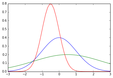
1p = plot(x, norm.pdf(x, loc=0, scale=1))
2p = plot(x, norm.pdf(x, loc=0.5, scale=2))
3p = plot(x, norm.pdf(x, loc=-0.5, scale=.5))
另一种则是将 loc, scale 作为参数直接输给 norm 生成相应的分布:
1p = plot(x, norm(loc=0, scale=1).pdf(x))
2p = plot(x, norm(loc=0.5, scale=2).pdf(x))
3p = plot(x, norm(loc=-0.5, scale=.5).pdf(x))

其他连续分布
1from scipy.stats import lognorm, t, dweibull
支持与 norm 类似的操作,如概率密度函数等。
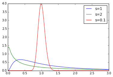
不同参数的对数正态分布:
1x = linspace(0.01, 3, 100)
2
3plot(x, lognorm.pdf(x, 1), label='s=1')
4plot(x, lognorm.pdf(x, 2), label='s=2')
5plot(x, lognorm.pdf(x, .1), label='s=0.1')
6
7legend()
<matplotlib.legend.Legend at 0x15781c88>
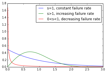
不同的韦氏分布:
1x = linspace(0.01, 3, 100)
2
3plot(x, dweibull.pdf(x, 1), label='s=1, constant failure rate')
4plot(x, dweibull.pdf(x, 2), label='s>1, increasing failure rate')
5plot(x, dweibull.pdf(x, .1), label='0<s<1, decreasing failure rate')
6
7legend()
<matplotlib.legend.Legend at 0xaa9bc50>
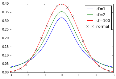
不同自由度的学生 t 分布:
1x = linspace(-3, 3, 100)
2
3plot(x, t.pdf(x, 1), label='df=1')
4plot(x, t.pdf(x, 2), label='df=2')
5plot(x, t.pdf(x, 100), label='df=100')
6plot(x[::5], norm.pdf(x[::5]), 'kx', label='normal')
7
8legend()
<matplotlib.legend.Legend at 0x164582e8>
离散分布
导入离散分布:
1from scipy.stats import binom, poisson, randint
离散分布没有概率密度函数,但是有概率质量函数。
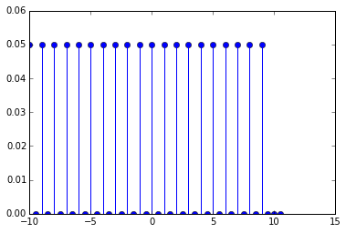
离散均匀分布的概率质量函数(PMF):
1high = 10
2low = -10
3
4x = arange(low, high+1, 0.5)
5p = stem(x, randint(low, high).pmf(x))  # 杆状图
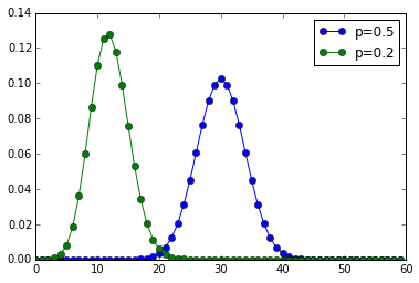
二项分布:
1num_trials = 60
2x = arange(num_trials)
3
4plot(x, binom(num_trials, 0.5).pmf(x), 'o-', label='p=0.5')
5plot(x, binom(num_trials, 0.2).pmf(x), 'o-', label='p=0.2')
6
7legend()
<matplotlib.legend.Legend at 0x1738a198>
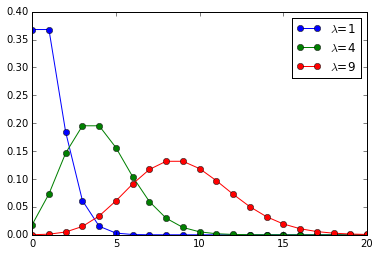
泊松分布:
1x = arange(0,21)
2
3plot(x, poisson(1).pmf(x), 'o-', label=r'$\lambda$=1')
4plot(x, poisson(4).pmf(x), 'o-', label=r'$\lambda$=4')
5plot(x, poisson(9).pmf(x), 'o-', label=r'$\lambda$=9')
6
7legend()
<matplotlib.legend.Legend at 0x1763e320>
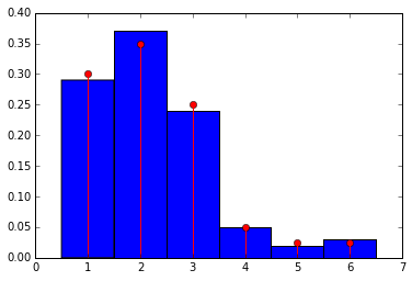
自定义离散分布
导入要用的函数:
1from scipy.stats import rv_discrete
一个不均匀的骰子对应的离散值及其概率:
1xk = [1, 2, 3, 4, 5, 6]
2pk = [.3, .35, .25, .05, .025, .025]
定义离散分布:
1loaded = rv_discrete(values=(xk, pk))
此时, loaded 可以当作一个离散分布的模块来使用。
产生两个服从该分布的随机变量:
1loaded.rvs(size=2)
array([3, 1])
产生100个随机变量,将直方图与概率质量函数进行比较:
1samples = loaded.rvs(size=100)
2bins = linspace(.5,6.5,7)
3
4hist(samples, bins=bins, normed=True)
5stem(xk, loaded.pmf(xk), markerfmt='ro', linefmt='r-')
<Container object of 3 artists>
假设检验
导入相关的函数:
- 正态分布
- 独立双样本
t检验,配对样本t检验,单样本t检验 - 学生
t分布
t 检验的相关内容请参考:
- 百度百科-
t检验:http://baike.baidu.com/view/557340.htm - 维基百科-学生
t检验:https://en.wikipedia.org/wiki/Student%27s_t-test
1from scipy.stats import norm
2from scipy.stats import ttest_ind, ttest_rel, ttest_1samp
3from scipy.stats import t
独立样本 t 检验
两组参数不同的正态分布:
1n1 = norm(loc=0.3, scale=1.0)
2n2 = norm(loc=0, scale=1.0)
从分布中产生两组随机样本:
1n1_samples = n1.rvs(size=100)
2n2_samples = n2.rvs(size=100)
将两组样本混合在一起:
1samples = hstack((n1_samples, n2_samples))
最大似然参数估计:
1loc, scale = norm.fit(samples)
2n = norm(loc=loc, scale=scale)
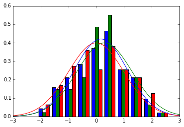
比较:
1x = linspace(-3,3,100)
2
3hist([samples, n1_samples, n2_samples], normed=True)
4plot(x, n.pdf(x), 'b-')
5plot(x, n1.pdf(x), 'g-')
6plot(x, n2.pdf(x), 'r-')
[<matplotlib.lines.Line2D at 0x17ca7278>]
独立双样本 t 检验的目的在于判断两组样本之间是否有显著差异:
1t_val, p = ttest_ind(n1_samples, n2_samples)
2
3print 't = {}'.format(t_val)
4print 'p-value = {}'.format(p)
t = 0.868384594123
p-value = 0.386235148899
p 值小,说明这两个样本有显著性差异。
配对样本 t 检验
配对样本指的是两组样本之间的元素一一对应,例如,假设我们有一组病人的数据:
1pop_size = 35
2
3pre_treat = norm(loc=0, scale=1)
4n0 = pre_treat.rvs(size=pop_size)
经过某种治疗后,对这组病人得到一组新的数据:
1effect = norm(loc=0.05, scale=0.2)
2eff = effect.rvs(size=pop_size)
3
4n1 = n0 + eff
新数据的最大似然估计:
1loc, scale = norm.fit(n1)
2post_treat = norm(loc=loc, scale=scale)
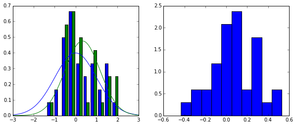
画图:
1fig = figure(figsize=(10,4))
2
3ax1 = fig.add_subplot(1,2,1)
4h = ax1.hist([n0, n1], normed=True)
5p = ax1.plot(x, pre_treat.pdf(x), 'b-')
6p = ax1.plot(x, post_treat.pdf(x), 'g-')
7
8ax2 = fig.add_subplot(1,2,2)
9h = ax2.hist(eff, normed=True)
独立 t 检验:
1t_val, p = ttest_ind(n0, n1)
2
3print 't = {}'.format(t_val)
4print 'p-value = {}'.format(p)
t = -0.347904839913
p-value = 0.728986322039
高 p 值说明两组样本之间没有显著性差异。
配对 t 检验:
1t_val, p = ttest_rel(n0, n1)
2
3print 't = {}'.format(t_val)
4print 'p-value = {}'.format(p)
t = -1.89564459709
p-value = 0.0665336223673
配对 t 检验的结果说明,配对样本之间存在显著性差异,说明治疗时有效的,符合我们的预期。
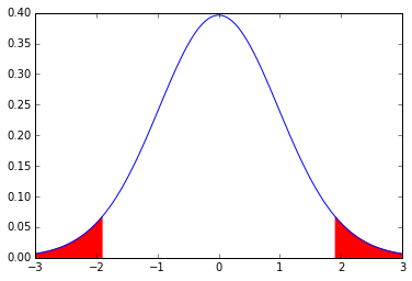
p 值计算原理
p 值对应的部分是下图中的红色区域,边界范围由 t 值决定。
1my_t = t(pop_size) # 传入参数为自由度,这里自由度为50
2
3p = plot(x, my_t.pdf(x), 'b-')
4lower_x = x[x<= -abs(t_val)]
5upper_x = x[x>= abs(t_val)]
6
7p = fill_between(lower_x, my_t.pdf(lower_x), color='red')
8p = fill_between(upper_x, my_t.pdf(upper_x), color='red')